Visualising demand forecast convergence using nemseer and xarray

In this example, we look at a couple of ways we can plot demand forecast convergence using a set of 5-minute pre-dispatch (5MPD or P5MIN) forecasts for the evening of 14/07/2022 for NSW. In particular, we’ll look at the ways to plot using xarray data structures.

Key imports

NEM data tools:

• NEMOSIS for actual market data

  • Data obtained from NEMOSIS is contained within pandas DataFrames

• NEMSEER for historical forecast data

  • In this tutorial, we focus on what we can do with data obtained from NEMSEER in xarray data structures

  • The xarray tutorial is a great resource for learning how to use xarray for data handling and plotting

Plotting

• matplotlib for static plotting. Both xarray and pandas have implemented plotting methods using this library.

• plotly for interactive plots. In some cases, we will use plotly directly, but in others, we will use hvplot.

• hvplot, a high-level API for plotting. hvplot can use many backends (default is bokeh, but we will use plotly) and makes it easy to plot xarray data structures using the .hvplot accessor

from pathlib import Path

import nemosis
from nemseer import compile_data, generate_runtimes


import plotly.graph_objects as go

import matplotlib.pyplot as plt

import hvplot.xarray
hvplot.extension("plotly")

# for some advanced colour manipulation
from matplotlib.colors import to_hex
import numpy as np

# plotly rendering
import plotly.io as pio
import plotly.express as px

INFO: generated new fontManager

Study times

Here we’ll define our datetime range that we’re interested in:

• NEMOSIS only accepts datetime strings with seconds specified.

• NEMSEER will accept datetimes with seconds specified, so long as the seconds are 00. This is because the datetimes relevant to NEMSEER functionality are only specified to the nearest minute.

(start, end) = ("2022/07/14 16:55:00", "2022/07/14 19:00:00")

Get demand forecast data for NSW

p5_run_start, p5_run_end = generate_runtimes(start, end,
                                             "P5MIN")
p5_data = compile_data(p5_run_start, p5_run_end, start, end,
                       "P5MIN", "REGIONSOLUTION", raw_cache="nemseer_cache/",
                       data_format="xr")
p5_region = p5_data["REGIONSOLUTION"]
# .sel() is a lot like .loc() for pandas
# We then use ["TOTALDEMAND"] to acces that specific variable
p5_demand_forecasts = p5_region.sel(
    forecasted_time=slice(start, end),
    REGIONID="NSW1"
)["TOTALDEMAND"]

Basic plotting with xarray

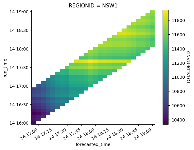
We can call .plot() on an xarray data structure to create a plot. Because our data is 3D (run_time, forecasted_time, TOTALDEMAND), xarray creates a heatmap.

p5_demand_forecasts.plot();

We can also create an interactive version using hvplot:

hvhmap = p5_demand_forecasts.hvplot.heatmap(
    x="forecasted_time", y="run_time", C="TOTALDEMAND"
)
# you can view this chart by calling the chart variable

Integrating actual demand into our plots

To compare forecasts with actual demand data, we will use NEMOSIS to obtain actual demand data for NSW for this evening.

# create a folder for NEMOSIS data
nemosis_cache = Path("nemosis_cache/")
if not nemosis_cache.exists():
    nemosis_cache.mkdir()

# get demand data for NSW
nsw_demand = nemosis.dynamic_data_compiler(
  start, end, "DISPATCHREGIONSUM", nemosis_cache,
  filter_cols=["REGIONID", "INTERVENTION"],
  filter_values=(["NSW1"],[0])
)
nsw_demand = nsw_demand.set_index('SETTLEMENTDATE').sort_index()

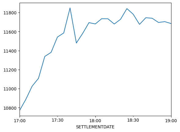
pandas has plotting functionality that wraps matplotlib:

nsw_demand["TOTALDEMAND"].plot();

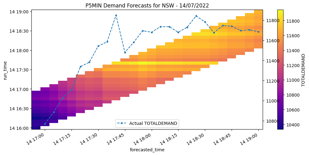
We’ll now tie the actual data in with our forecasted data. The actual data will be a line chart, and the forecast data will be a heatmap. We’ll first do this using matplotlib:

1. Create a matplotlib axis

2. Plot out heatmap onto this axis

3. Then create a secondary y-axis (via ax.twinx()) and plot our actual demand

fig, ax = plt.subplots(1, 1, figsize=(12, 5))
p5_demand_forecasts.plot(cmap="plasma", ax=ax)
ax_demand = ax.twinx()
ax_demand.plot(nsw_demand.index, nsw_demand["TOTALDEMAND"], ls="--", marker=".",
               label="Actual TOTALDEMAND")
ax_demand.legend(loc="lower center")
ax.set_title("P5MIN Demand Forecasts for NSW - 14/07/2022");

Faceted Plotting

The forecast that was run at the same time as a demand spike seems to forecast relatively high demand when compared to adjacent forecast runs. Let’s see if we can make that a bit clearer.

We’ll create a set of faceted plots that separate different runtimes to look at this closely.

# This creates an xarray FacetGrid
fg = p5_demand_forecasts.plot(hue="run_time", col="run_time", col_wrap=4)
# We then iterate through the matplotlib axes to add the actual data
for ax in fg.axes.flat:
    ax.plot(
        nsw_demand.index, nsw_demand["TOTALDEMAND"], label="Actual", ls="--", color="gray"
    )
    ax.legend()
fg.set_ylabels("TOTALDEMAND (MW)");

/tmp/ipykernel_687/95342703.py:4: DeprecationWarning:

self.axes is deprecated since 2022.11 in order to align with matplotlibs plt.subplots, use self.axs instead.

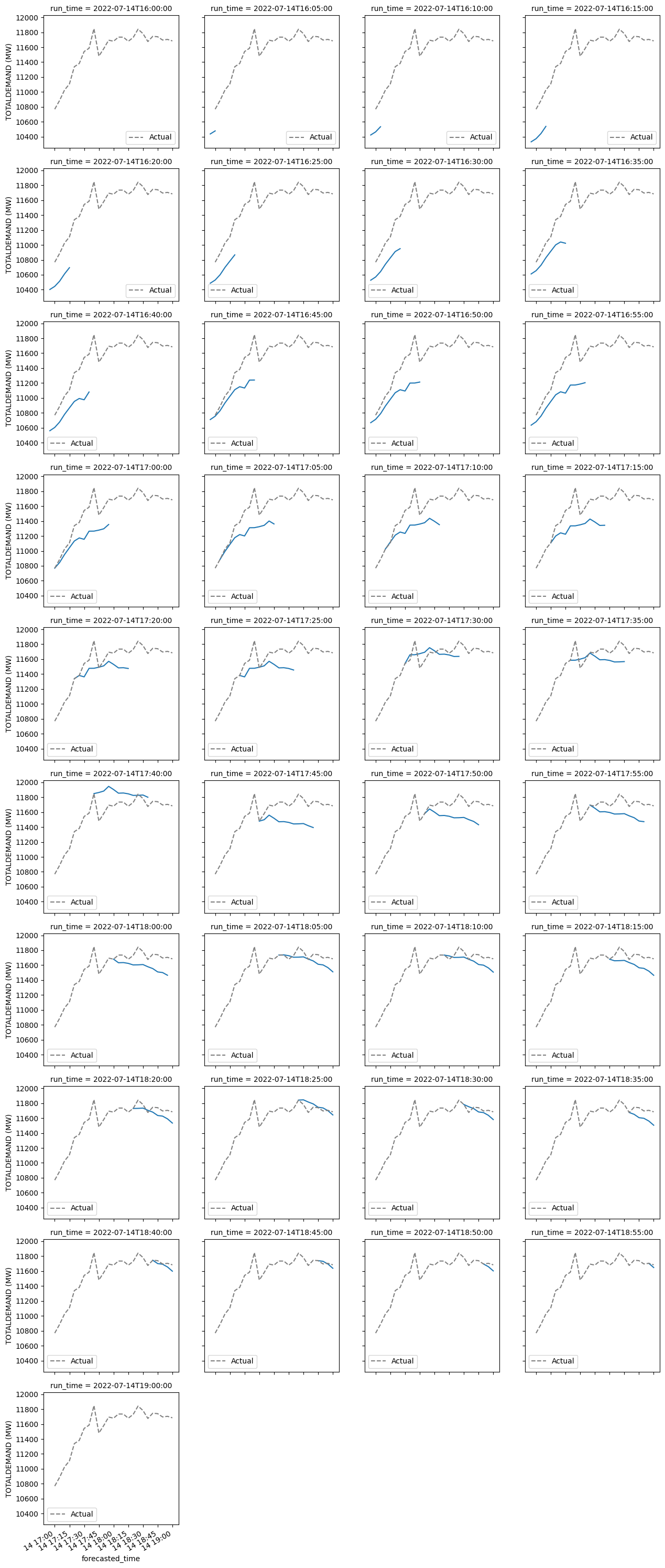
From this, it’s a little clearer that demand forecasting for 5MPD is heavily influenced by current demand. In actual fact, demand forecasts for the last 11 dispatch intervals in a 5MPD forecast are based on a recursive application of an average percentage demand change, which is specific to a given dispatch interval and whether the day is a weekday or weekend. This average percentage demand change is calculated using demand data form the last two weeks. For more information, see this AEMO document on 5MPD demand forecasting and this AEMO document on demand terms in the EMMS data model.

Interactive Plots

Now we’ll try and recreate some of the plots above using plotly.

hvplot helps us generate the chart we need from the xarray data structure. After that, we need to obtain a plotly object to work with to add additional traces.

# Generate interactive heatmap
hmap = p5_demand_forecasts.hvplot.heatmap(
    x="forecasted_time", y="run_time", C="TOTALDEMAND", cmap="plasma",
    title="P5MIN Demand Forecasts for NSW - 14/07/2022"
)
# Create plotly.go.Figure from hvplot data structure
fig = go.Figure(hvplot.render(hmap, backend="plotly"))
# add actual demand as a line trace
line = go.Scatter(
    x=nsw_demand.index, y=nsw_demand["TOTALDEMAND"], yaxis="y2",
    line={"color": "black", "dash": "dash"}, name="Actual TOTALDEMAND",
    )
fig.add_trace(line)
# update_layout defines the second y-axis and figure width and height
fig = fig.update_layout(
    xaxis=dict(domain=[0.1, 0.9]),
    yaxis2=dict(overlaying="y", title="Actual TOTALDEMAND (MW)", side="right"),
    height=300, width=700
)
# you can view this chart by calling the chart variable
# below, we load a pre-generated chart

hvplot has easy ways to integrate interactivity. We can trigger this by leaving one dimension as a degree of freedom (e.g. specifying x-axis as forecasted_time, y-axis as TOTALDEMAND thus leaving run_time as a degree of freedom).

We can also get hvplot and plotly to plot across the degree(s) of freedom simultaneously using by=:

run_time_iterations = p5_demand_forecasts.hvplot(by="run_time")
run_lines = go.Figure(hvplot.render(run_time_iterations, backend="plotly"))
# you can view this chart by calling the chart variable
# below, we load a pre-generated chart

This is quite hard to read. We can clean this up and use a sequential colour scheme to indicate forecast outputs from later run times:

# obtain data from hvplot
plotly_data = hvplot.render(run_time_iterations, backend="plotly")
# modify the colour of each trace using the Reds sequential colormap
for i, increment in enumerate(np.linspace(0, 1, len(plotly_data["data"]))):
    plotly_data["data"][i]["line"]["color"] = to_hex(plt.cm.Reds(increment))
# create a plotly.go.Figure
overlay = go.Figure(plotly_data)
# add actual demand data
line = go.Scatter(
    x=nsw_demand.index, y=nsw_demand["TOTALDEMAND"], yaxis="y2",
    line={"color": "black", "dash": "dash"}, name="Actual TOTALDEMAND",
    )
overlay.add_trace(line)
# update the layout to specify the secondary y-axis
overlay = overlay.update_layout(
    xaxis=dict(domain=[0.1, 0.9]),
    yaxis2=dict(overlaying="y", title="Actual TOTALDEMAND (MW)", side="right"),
    height=300, width=700,
    title = "P5MIN Demand Forecasts for NSW - 14/07/2022"
)
# you can view this chart by calling the chart variable
# below, we load a pre-generated chart